This post is an adaptation of one of my academic works as an Aerospace Engineering student at the Technical University of Munich. I produced this thesis as part of a six-month working student position at the German Aerospace Center (DLR). This post summarizes my thesis and presents some of the results in a less technical fashion. This summary provides an overview of laser space communication, sensor calibration, test design, and C++ and Matlab programming.
What follows is the official title and abstract of the thesis as submitted to the university.
Calibration of MEMS Accelerometers for Vibration Sensing in CubeSat Laser Communication Terminals
Recent trends in the development of modular and compact satellite systems such as laser communication terminals include the use of commercial off-the-shelf components such as MEMS accelerometers for micro-vibration sensing due to their advantages of low cost, compactness, and light weight.
This work investigates MEMS accelerometers by characterizing this sensor and comparing it with reference data to derive a system characteristic function that can be used for sensor calibration to improve sensing accuracy.
High-end vibration equipment and software are used to obtain back-to-back MEMS and reference vibration data from a controlled shaker platform excitation. Excitation methods investigated include stepped sinusoidal, chirp sinusoidal, and random oscillations.
Time and frequency domain processing allows direct comparison and analysis of the acceleration frequency response of the MEMS accelerometer.
The test setup demonstrated the ability to generate qualitative data with satisfactory MEMS accelerometer accuracy even prior to calibration.
The calibrated signal improves the correlation coefficient deviation to the reference data compared to the uncalibrated signal from about 17% to 1% across 98% of the selected frequency bandwidth.
The data obtained in this study supports the introduction of this type of sensor for vibration sensing in optical communication terminals, showing that it fits the broader concept of compact and modular systems and still provides sensor quality with or without calibration.
Additional characterization:
A characterization of the Falcon 9 launch loads and end-of-life radiation effects on the MEMS sensor shows that these environments do not degrade the characteristics of the MEMS sensor, ensuring that the calibration will remain accurate over the lifetime of the satellite.
Introduction
This post aims to highlight some of the contributions to the broader efforts in validating attitude control and estimation algorithms for free space optical communications in the context of the next CubeSat missions conducted by the Institute of Communications and Navigation at the German Aerospace Center (DLR).
The objective is to investigate and characterize the vibrations and microvibrations generated by the Laser Communication Terminal as part of the satellite system during operation in orbit. To acquire this data, an accelerometer must be integrated into the system. The chosen accelerometer is a MEMS accelerometer incorporated into the Master Attitude Controller (MAC) board. Accurate measurements are essential for the success of this task, so the MEMS accelerometer sensor must be calibrated on the ground before being sent into orbit.
This summary explains the efforts that resulted in the characterization and calibration of the sensor as well as the methodologies used and the test setup. The results obtained will improve the understanding of the vibration environment generated while the optical terminal operates in orbit and provide data for improving optics design.
The context, before we start
Here’s a quick introduction to some of the central topics my thesis touched on.
Space Optical Communications
Optical communication offers advantages over traditional communication systems in many ways. Free space optical communications using laser beams enables high data rate transmission through air, vacuum or outer space. As a result, this technology has been implemented in inter-satellite links and ground-to-satellite or satellite-to-ground applications. Optical communications are emerging as a viable alternative to traditional radio frequencies, offering superior data rate capabilities, fewer regulatory constraints and reduced size, weight and power (SWaP) requirements.
Small Satellites
In recent years, there has been significant growth and expansion of small satellite solutions, starting in the 2000s and increasing sharply in the 2010s. This recent trend is being driven by commercial entities seeking flexibility, low costs, and rapid development. Following this new tendency, governments are interested as well. A significant benefit of leveraging advancements in microelectronics is reduced construction, testing, and deployment costs. This makes it easier to establish communication and internet constellations, such as SpaceX’s Starlink, Amazon’s Kuiper, and OneWeb, as well as observation constellations, resulting in increased geodetic activity.
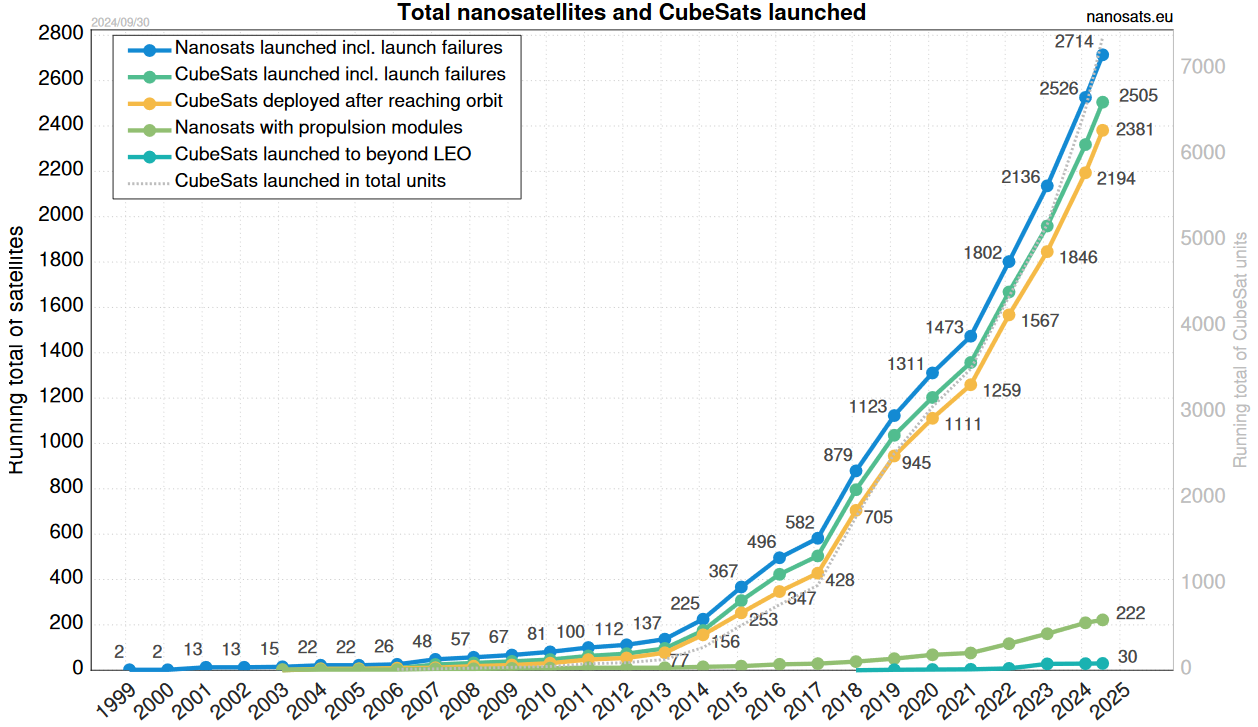
Total number of small satellites launched up to the end of 2024.
Source: nanosats.eu
Mems Accelerometers
With the advent of the New Space phenomenon, the industry is shifting towards shorter qualification and development times, modular designs, and commercial off-the-shelf (COTS) components. These components are ideal for short CubeSat missions (around five years) because they are inexpensive and often surpass the state of the art of more traditional, fully space-qualified components. A good example of this is MEMS accelerometers. These are the type of sensors that require calibration along their frequency range for on-orbit operation.
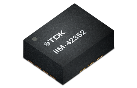
An example of a MEMS accelerometer. Its compact dimensions (2.5mm x 3mm x 0.91mm) make it useful for multiple applications.
Source: “IIM-42352 Datasheet” (2022)
Micro-electro-mechanical system (MEMS) sensors are widely used because they can accurately measure vibrations and are inexpensive, low-power, and compact. Circuit miniaturization and advanced manufacturing using microelectronic fabrication techniques make these sensors possible. These technologies combine microscopic mechanical sensing structures with microelectronic circuits to deliver these small yet accurate devices.
There is literature regarding the use of MEMS accelerometers in space, particularly for navigation and vibration sensing purposes. This speaks to the effectiveness of these sensors for space applications. However, it was also observed that recorded MEMS data generally deviates from reference data. This phenomenon originates from the operating principle of MEMS accelerometers and is an inherent characteristic of the technology. This kind of problem is precisely what this work addresses.
So, what’s the deal?
A step-by-step description of the accelerometer frequency calibration process, along with the necessary code for replication, is lacking in the literature. That’s why I did it.
Test Setup
An experiment is designed to accurately compare the reference and MEMS accelerometers. The experiment uses VibrationResearch’s VR9500 controller with VibrationVIEW software connected to a Controlled Vibration EDP-1818 shaker via two Crown XLS 1002 power amplifiers. This setup is shown in figure below. On the shaker, the two accelerometers are mounted on a plate specially designed and manufactured for this test series. The plate acts as an interface between the imperial units of the table and the metric units of the PCB. In addition, the plate acts as a mounting surface for the reference accelerometer. The reference accelerometer is a PCB Piezotronics Model 355B04 and is periodically calibrated, therefore the data generated by this accelerometer can be considered accurate.
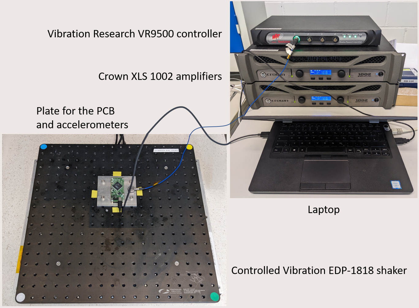
The setup for the experiments. Top right, the VR9500 controller on top of the Crown XLS 1002 power amplifiers with the laptop used for the test recordings. Bottom left, the Controlled Vibration EDP-1818 shaker. Mounted on it is the realized plate for mounting the MAC PCB and the reference accelerometer.
The VR9500 controls the shaker through a direct connection to the reference accelerometer. Therefore, the data generated by the reference accelerometer can be viewed and analyzed in VibrationVIEW. The VibrationVIEW license held by DLR in conjunction with this particular VR9500 controller was not allowing raw time data to be recorded by VibrationVIEW. Only secondary data such as the G-peak amplitude could be analyzed. Since the MEMS accelerometer generates the raw time data, a direct comparison was not possible. For this reason, some initial tests were developed in an attempt to not use the reference raw time data, resulting in the Stepped-Sine approach presented in the thesis. After it became clear that for a better and direct comparison of the same quantities, the raw time data of the reference accelerometer was also needed, an additional license for RecorderVIEW was used to enable the direct raw time recording in VibrationVIEW.
The MEMS accelerometer is integrated onto the MAC on the PCB, which is mounted on the plate next to the reference accelerometer. Therefore, the MEMS accelerometer can only be controlled by C++ software sent from a laptop. Due to this limitation, which results in two different data acquisition methods, a perfectly synchronized operation and recording of the two accelerometers is impossible. This means that the signals must be aligned during data processing, adding a further layer of complexity to the data analysis.
To define the frequency band of interest, a sampling frequency of 4000 Hz is chosen. This allows the acceleration data to be acquired and calibrated in the frequency band up to 2000 Hz according to the Nyquist-Shannon sampling theorem. Higher sampling frequencies were considered (according to the data sheet, the IIM-42352 MEMS accelerometer is capable of measurements up to 32 kHz) to provide better sampling accuracy or to increase the frequency band of interest. With some tests using an oscilloscope and setting the pins on the PCB to high and low states to measure how the MAC microcontroller performs its various functions such as acceleration measurement and sampling, it was verified that a higher sampling frequency would overload the microcontroller. In addition, because of the use case for this particular MEMS accelerometer, higher frequencies are not of interest for its later operation in space.
Microcontroller C++ programming
As mentioned previously, the only way to record data from the MEMS sensor integrated into the Master Attitude Controller PCB was through C++ code and a terminal. For this reason, a new state was integrated into the MAC’s software.
The C++ code is structured as follows:
- Creation of the header for terminal or log file output.
- When new data is ready, it is measured and saved. Due to the large quantity of data generated, the function that saves to flash memory had to be coded. This was essential, as the internal memory available was insufficient for the data generated during each session.
- Only after the entire recording session is complete will the output be generated and written to the terminal or log file. Separating the writing process from the measurement phase reduces the microprocessor’s workload during measurement. It has been observed that this approach eliminates artifacts and overflow errors.
Step 1: Accelerometer characterization
After the test setup is validated, it is necessary to collect data about the accelerometer before the calibration.
There are multiple approaches and analyses carried out in my thesis regarding the characterization of the MEMS accelerometer. These include vibration approaches, such as the stepped sinusoidal, chirped sinusoidal and random approaches, as well as an analysis of the Falcon 9 launch loads and the end-of-life radiation impacts on the calibration itself.
Of all the characterizations mentioned in this post, only the chirp sinusoidal (or sweep sine) excitation is presented since it is used for calibration.
For this test, a Chirped-Sine excitation was programmed in VibrationVIEW. The following table shows the two most important parameters selected for this test.
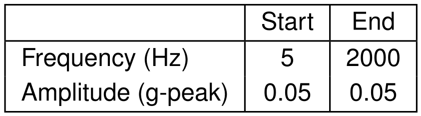
Frequency and amplitude profile for the chirp sinusoidal excitation.
A logarithmic sweep rate of 18 octaves per minute (oct/min) was chosen. This results in a recording time of less than 45 seconds, ensuring the recording would not generate an excessive amount of data. The sweep rate determines the rate at which the frequency increases (or decreases) over time.
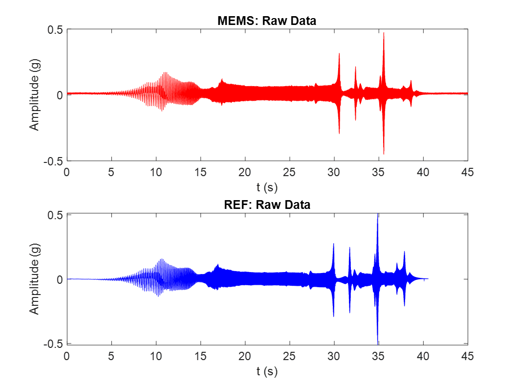
Signals in time domain
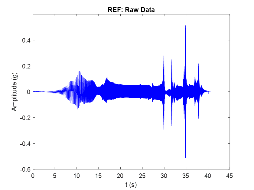
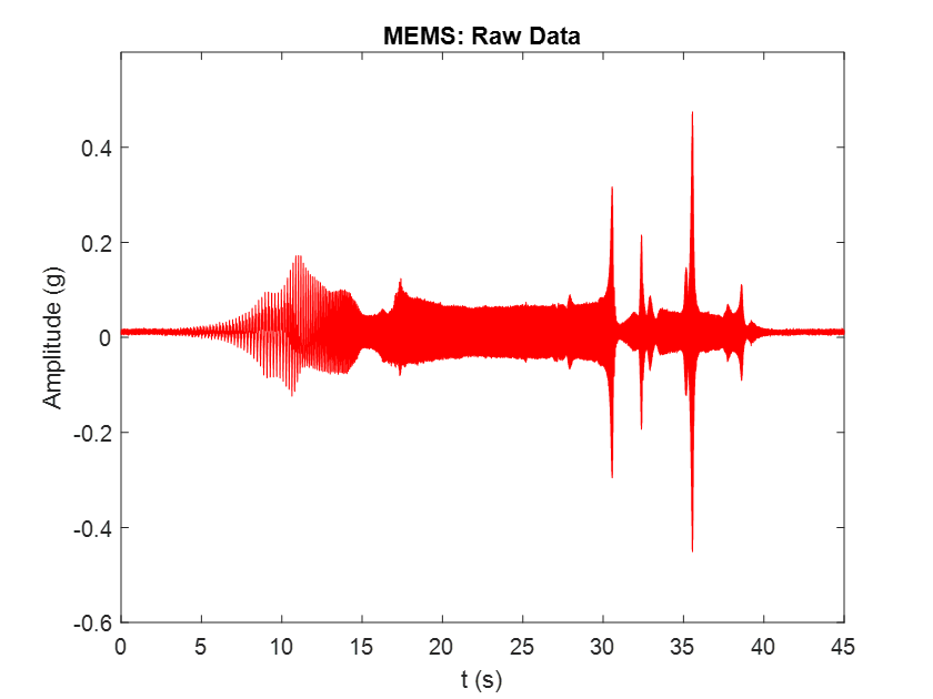
The figures below show the time-domain acceleration outputs generated by the reference and MEMS sensors without any signal processing.
|
|
On the left: Reference accelerometer raw time data for the chirp sinusoidal excitation. On the right: MEMS accelerometer raw time data for the chirp sinusoidal excitation.
Upon first glance, the two signals appear very similar, with only minor differences in peak amplitude. Due to the test constraints explained above and the different recording methods used for the two sensors, it is not possible to start the two signals exactly at the same time. Therefore, the signals must be accurately aligned prior to comparison.
Signals in frequency domain
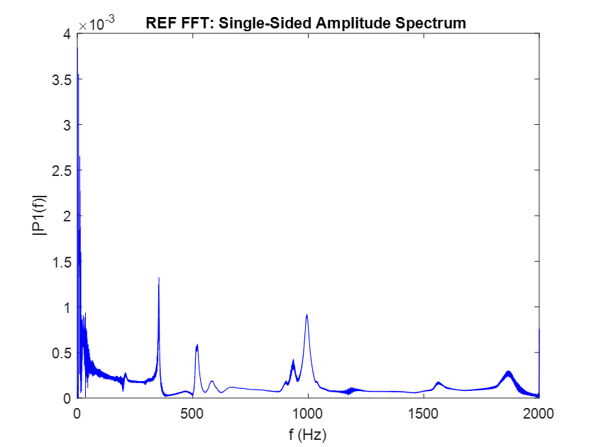
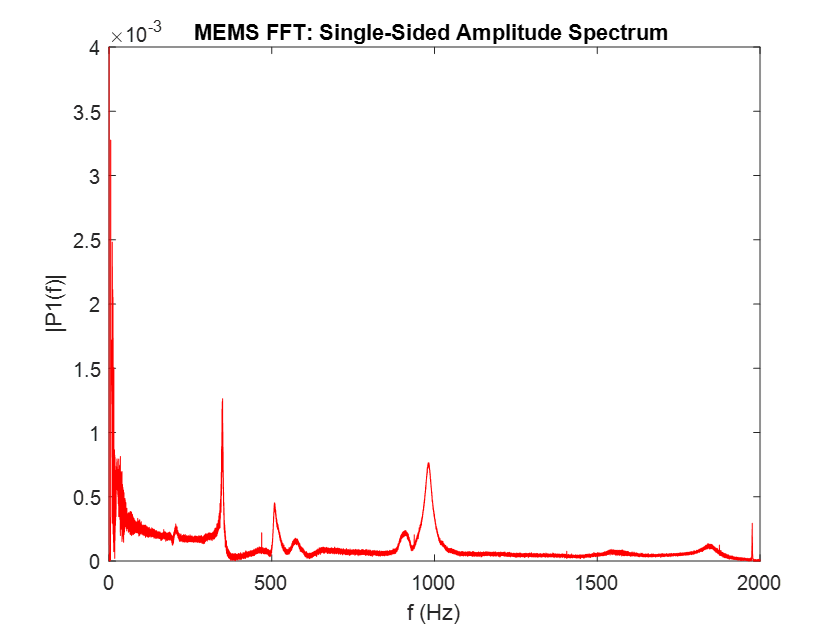
To further analyze the signals and compare them also in the frequency domain, a Fast Fourier Transform (FFT) is performed, which yields again similar results for both accelerometers, as shown in the figures below.
|
|
On the left: Reference accelerometer raw time data for the chirp sinusoidal excitation. On the right: MEMS accelerometer raw time data for the chirp sinusoidal excitation.
Ignoring the peak occurring at 0 Hz, which is attributable to the DC-Offset in sensor positioning along the gravity vector, a slight difference in the intensity of the excitation appears in the second half of the bandwidth. Here, the red MEMS curve is found to be below the level of the blue reference curve. This discrepancy can be corrected in the calibration process.
Power spectograms
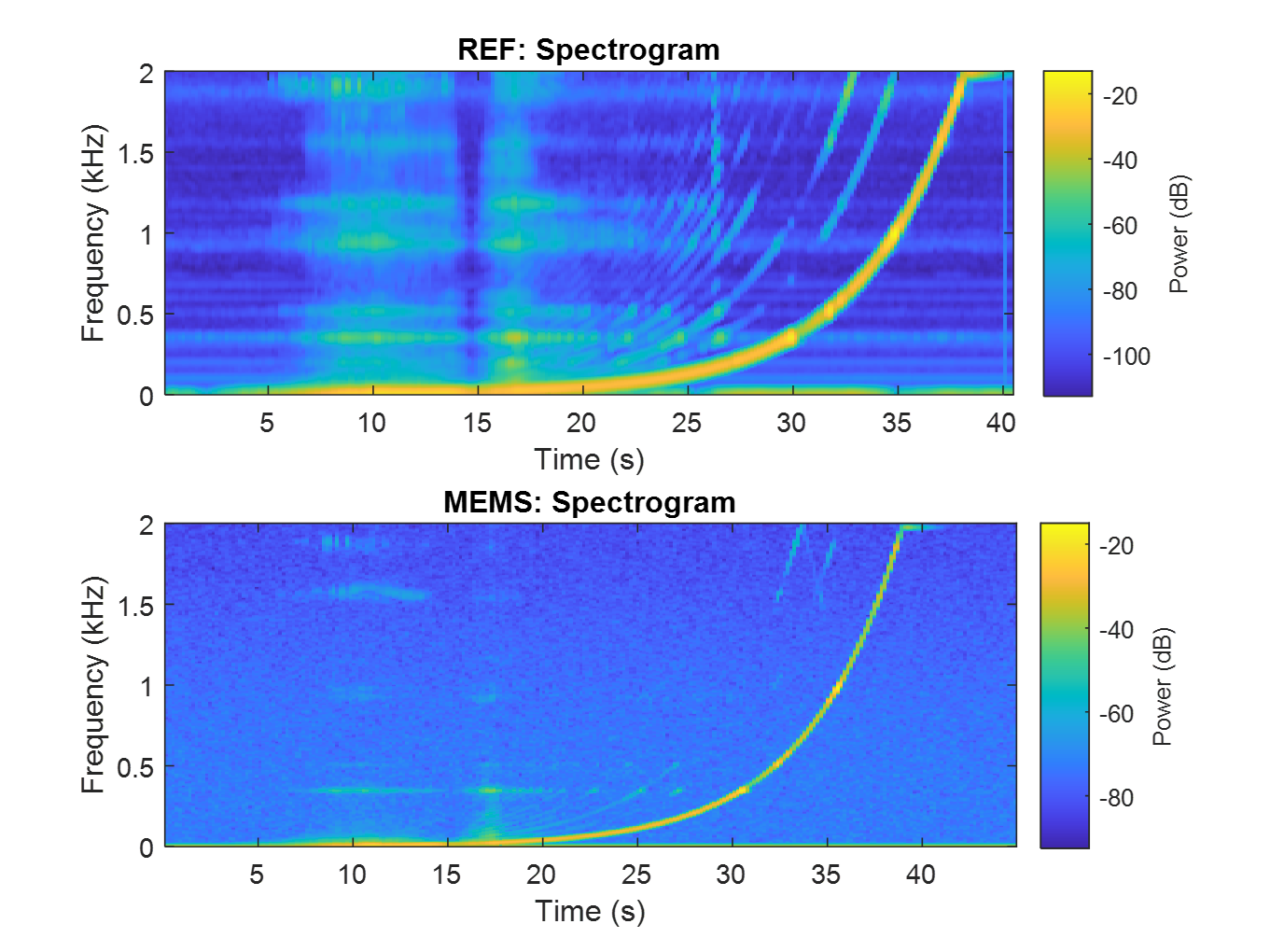
Another type of plot that can help visualize the chirped-sine excitation recorded by the two sensors is the Power Spectrogram. The following figures show the power spectrogram of the signals in 2D and 3D plots, respectively.
|
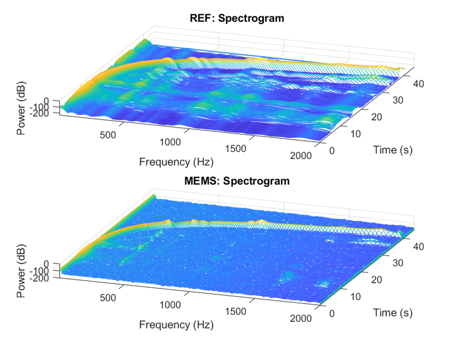
|
On the left: Power Spectrum 2D plots for reference and MEMS accelerometers showing the chirp sinusoidal power response over the frequency and time. On the right: Power Spectrum 3D plots for reference and MEMS accelerometers showing the chirp sinusoidal power response over the frequency and time.
The power curve resulting from a logarithmic sweep rate is clearly visible in both plots for both sensors and aligns with the selected parameter of 18 octaves per minute (oct/min), as mentioned above. The reference accelerometer’s lower signal noise is evident in the darker blue shades in the image, when compared to the MEMS signal. This is to be expected, as MEMS accelerometers are known to have a higher noise-to-signal ratio than more expensive, larger alternatives. These plots also highlight the need for signal alignment for the upcoming sensor calibration, as can be seen by looking at the time axis and the progression of the power curves.
This type of graph shows that the sensors measured the type of chirped-sine excitation they were subjected to. It also supports the other graphs in this section, such as the time- and frequency-domain excitation plots. Thus, the produced data can be used for calibration, with the knowledge that the generated data behaves as expected.
Step 2: Accelerometer calibration
This chapter describes the steps required for MEMS accelerometer calibration, from data import and preprocessing to calculation of the characteristic function.
As is commonly done in the literature, for this part the data obtained with the chirp-sine excitation approach is used. Data from both sensors is prepared for import into MATLAB using Microsoft Excel and exported as a .CSV file.
For the MEMS accelerator, data that is generated directly through the Visual Studio Code terminal using the debugging feature is stored in a log file in .TXT format.
The text file is then modified in Excel by removing the header and footer. Then, an elapsed time column is added, and the acceleration is scaled to 0 g to allow comparison with the reference data. The gravitational vector causes the MEMS accelerometer to register a constant acceleration of 1 g on Earth. However, this is not the case in orbit under microgravity conditions.
For the reference accelerometer, data recorded through the VibrationVIEW suite can be exported directly from ObserVIEW as a .CSV file. Minor adjustments were necessary, such as removing the header and footer notes.
The Matlab code written to perform the calibration can be used to calibrate any other accelerometer, if the correct input data format is provided.
As input, the code requires two .CSV files: one for the accelerometer to be calibrated and one for the reference accelerometer. The .CSV file for each accelerometer must contain acceleration data organized into two columns: the first column contains the elapsed time in seconds, and the second column contains the acceleration in g. The code automatically synchronizes the accelerometers and cleans and normalizes the data.
As output, the calibration function is generated, and plots of the uncalibrated and calibrated data are displayed. The next paragraphs will show these results.
Raw data import and preprocessing
The raw data from the accelerometers is plotted in the figure below on the left to illustrate the starting point of the calibration process. The following preprocessing operations are performed, resulting in the signals displayed in the figure on the right:
- Alignment in the time axis. The accelerometers are synchronized.
- Alignment in the acceleration axis. The constant (at 0 Hz) gravitational offset (DC offset) generated by the accelerometer’s positioning on the plate is corrected.
- Resampling to the MEMS sampling frequency due to the different frequencies at which the signals were recorded.
- Trimming to the same signal length to ensure that the vector and matrix dimensions are compatible in Matlab, allowing the calculation to be performed.
|
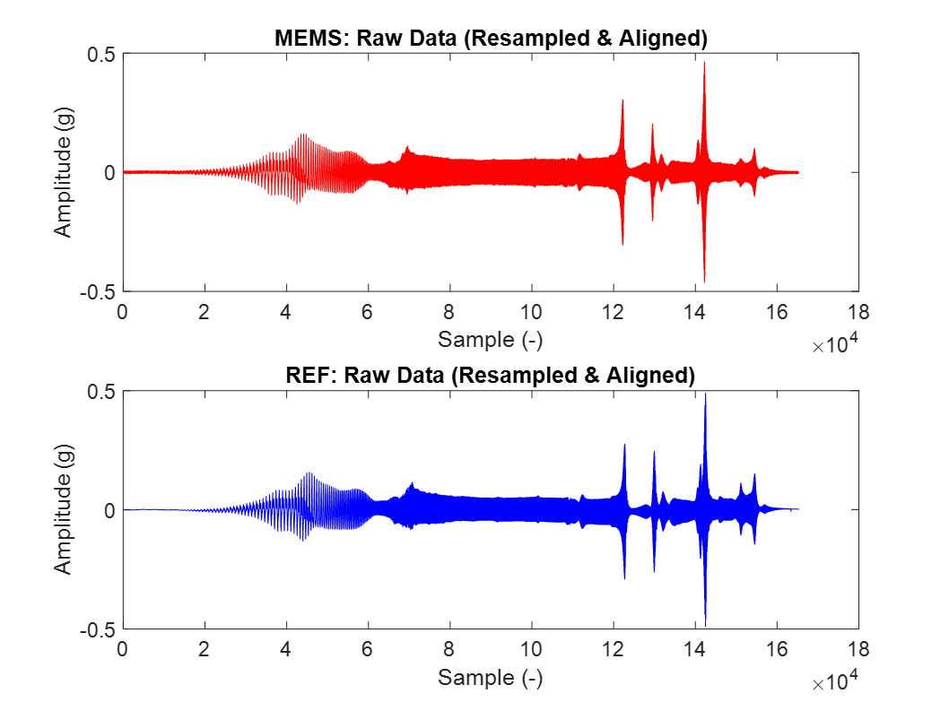
|
On the left: Raw data recorded by reference and MEMS accelerometers. On the right: The same raw data after time and amplitude axis alignment, resampling and trimming.
A more detailed explanation on the steps (1.)-(4.) is provided below.
-
As explained before regarding the experimental setup, two different methods were used to record data from the two accelerometers. Therefore, when subjected to the same vibration, the two accelerometers recorded the data with slight differences in elapsed time. This introduces the challenge of timing the two signals to allow for comparison. Since it is impossible to perfectly synchronize the start of the recording for both accelerometers during the test, synchronization is performed in the code by aligning the signals in the time domain. For this purpose, the cross-correlation algorithm is used. Widely used in pattern recognition, the cross-correlation algorithm measures the similarity of two signals as a function of their relative displacement.
-
Continuing on the topic of alignment, the acceleration axis is addressed by examining the offset generated by the sensor’s positioning, also known as the DC offset. The DC offset is the amount of acceleration detected when the accelerometer is not excited. In an experimental setting, the main cause is the accelerometer being positioned so that the sensing axis is not aligned with the excitation axis. This can be attributed to the leveling of the PCB, mounting plate, shaker, or floor. Even if the initial data did not have a significant offset, the DC shift is removed.
-
Addressing a further challenge generated by the use of two different sensors with two different data acquisition methods, the topic of sampling frequency is examined. Due to the constraints in sampling requirements for the MEMS accelerometer and the VibrationView software for the reference accelerometer, a common sampling frequency could not be selected for this setup. Therefore, when recording at two different frequencies, the data must be resampled to a common value. To avoid creating fictitious data, it is recommended to resample each signal at the lower sample rate. The resample command is applied to both signals due to the addition of an anti-aliasing low-pass filter, which compensates for the introduced delay. To provide a sense for the scale of the generated data, the sampling frequencies used are given. The sampling frequency selected for the MEMS accelerometer is 4 kHz. The minimum sampling frequency available in VibrationVIEW for the Chirp-Sine mode is 10 kHz. With approximately 45 seconds of recording time, the generated .CSV files already exceed the size of tens of megabytes. This creates additional challenges, such as Microsoft Excel’s inability to process data once the maximum number of rows in a file is exceeded, as well as increased compile and run times in Matlab.
-
The final step in the preprocessing stage is trimming both signals to the last common sampled bit. At the end of the preprocessing process described in these paragraphs, perfectly aligned signals are obtained which are trimmed to same length and dimensions, and ready for subsequent steps.
System’s characteristic function
A characteristic function, also known as a transfer function, describes the relationship between a system’s output and its input. This means that for a given system, the difference between each input applied to the system and its corresponding output is always the same function. Thus, the transfer function only needs to be characterized once to calculate an input given any output, or vice versa.
This property will be used to calibrate the MEMS accelerometer, which is generating an output based on the input recorded by the reference accelerometer. To illustrate the principle of operation of a transfer function, a simple schematic is presented in which the transfer function is treated as a black box. As shown in the figure below, an input is transformed into an output.
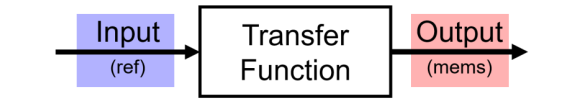
Transfer function (characteristic function) diagram with input (reference data) and output (MEMS data) signals.
Assigning the role of input to the calibrated reference accelerometer and the role of output to the MEMS accelerometer makes it possible to estimate, through the transfer function, the deviation of the uncalibrated MEMS accelerometer from the calibrated data. The inverse of this quantity can be applied to the MEMS data to achieve calibrated data. The characteristic function is calculated by dividing the output by the input. This is displayed qualitatively below.
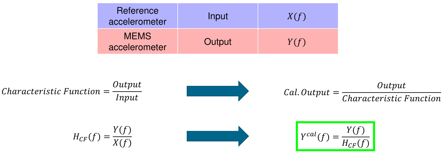
The genesis of the characteristic function using simple arithmetic.
For the case taken into consideration here, calculating the transfer function means dividing the MEMS preprocessed data by the reference preprocessed data. This calculation is performed in Matlab using the tfestimate() function, and the resulting plot is shown below.
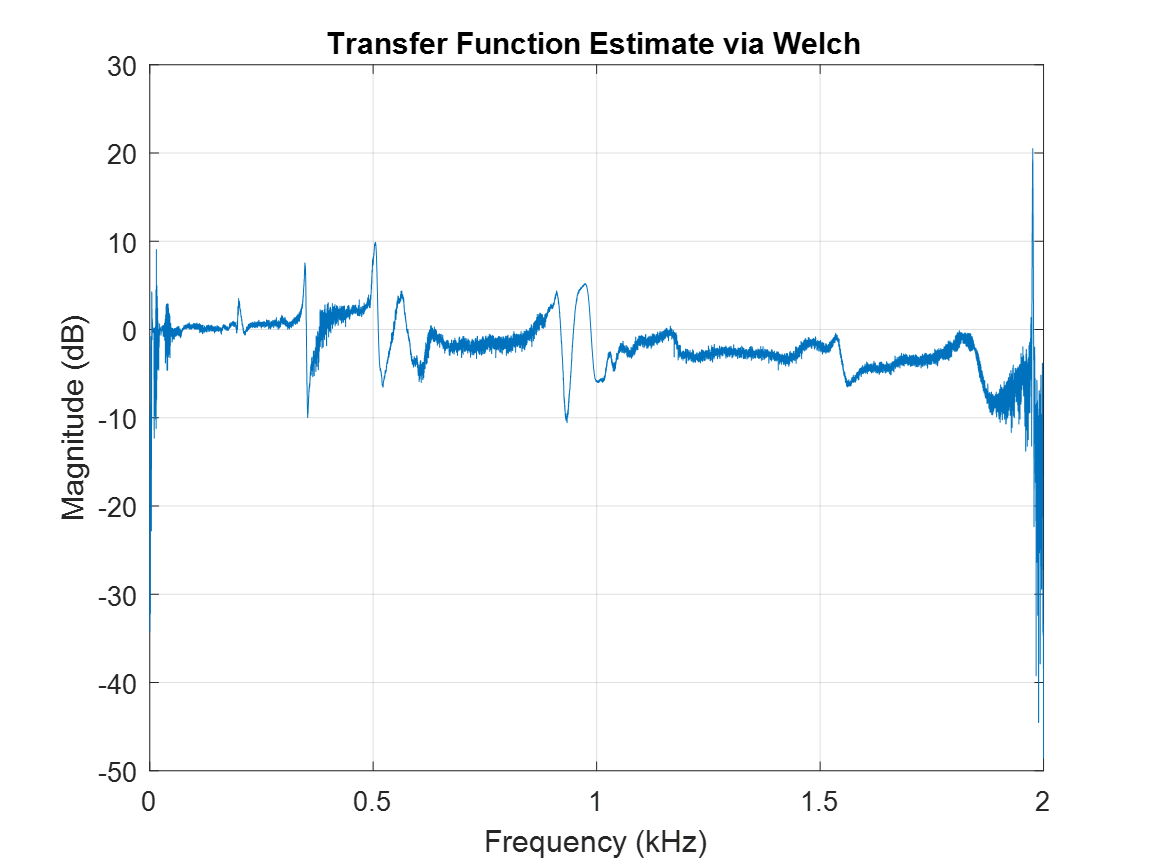
Transfer function estimation by Welch’s method computed in Matlab using the tfestimate() function.
The illustration of the system’s Transfer Function reveals the following notable features:
- In general, a stable and flat response is evident across the entire frequency bandwidth recorded by the MEMS accelerometer. This means that the MEMS accelerometer and the whole test setup acquired good data.
- A decrease in magnitude is observable, particularly after the first half of the bandwidth. This means that the difference in magnitude recorded by the two data streams increases as the signal frequency rises.
- Some frequencies experience spikes in both the positive and negative decibel directions due to potential inaccuracies.
- At the beginning and particularly at the end of the bandwidth, the transfer function appears unstable, and the two recorded signals diverge.
A similar analysis was performed on the Frequency Response Function (FRF), but it has been excluded here since it is too intricate given the scope of this post.
Step 3: Calibration results and quantifying the improvements
Before calibration
Before examining the effectiveness of the calibration, let’s review the comparison prior to calibration in the following figure.
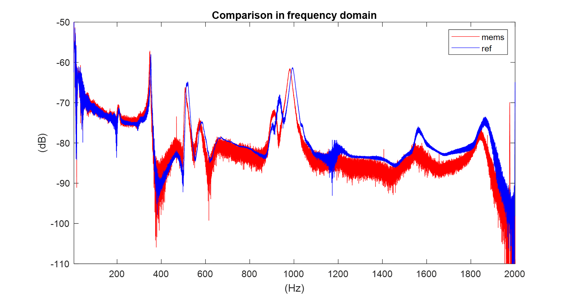
Acceleration curves of MEMS accelerometer and reference accelerometer prior to calibration.
It is already noticeable how accurate and concordant the recorded data is compared to the reference. One feature that immediately catches the eye is the difference in noise in the signals. The reference sensor, which is a dedicated sensor designed for these kinds of tests, generates a much cleaner curve. The MEMS sensor, which is much more compact and PCB-integrated, shows a higher Noise-to-Signal Ratio. In the second half of the frequency bandwidth, an offset buildup is visible. An interesting region to investigate after calibration is around the 1000 Hz frequency. Here, the two curves differ, making it a good area to observe the effects of calibration.
After calibration
The result of the calibration is shown in the following figure.
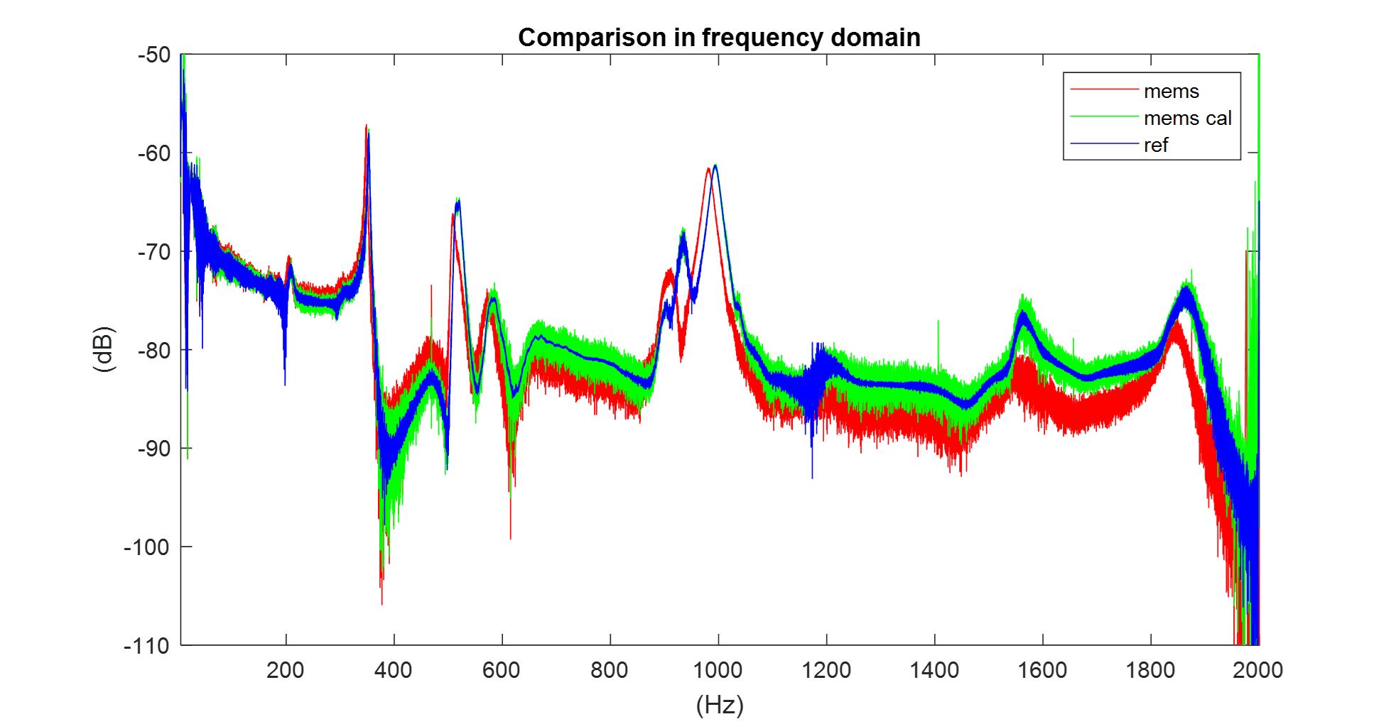
Acceleration curves of MEMS accelerometer and reference accelerometer after calibration.
After calibration, the green curve follows the blue reference curve much more closely across the entire frequency range, providing data that is more consistent with that of the reference accelerometer. Obviously, the noisier characteristic is maintained, as that is in the nature of the MEMS sensor, but the better fit to the reference data is significant.
Now, overlaying the coherence of the signals in the comparison reveals additional features worth discussing. This is presented in the following figure.
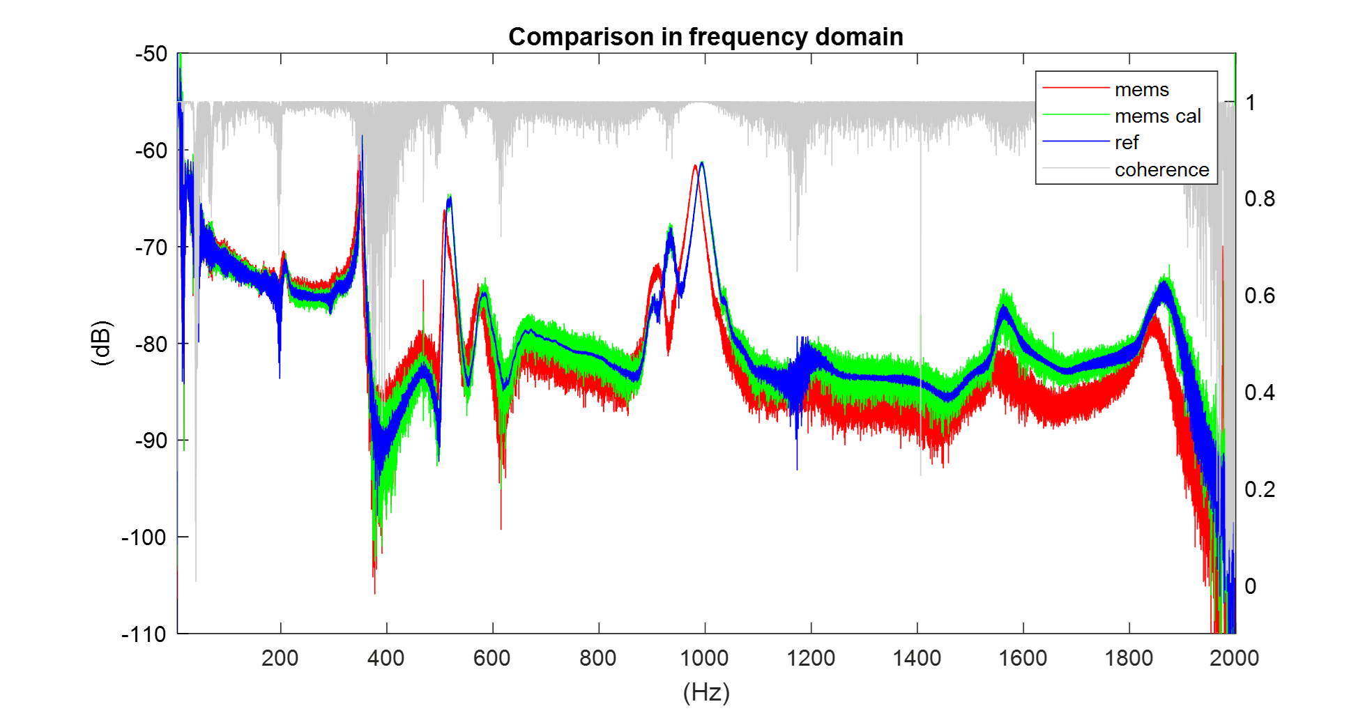
Acceleration curves of MEMS accelerometer and reference accelerometer prior to calibration. Added signal coherence values.
Generally speaking, a higher coherence value corresponds to better calibration, as suggested by the plot. This is evident around the 1000 Hz mark, where the calibration perfectly aligns with the reference curve. Another noteworthy feature of the plot is the low coherence values observed at frequencies around 370 Hz. This can be explained by the test setup: the shaker platform was placed on the floor on bubble mounts (small vibration dampeners). Since the shaker was not bolted down to the floor, when its resonance frequency was reached, the only way to prevent the excitation from aborting due to the control value was the control algorithm itself. This made acquiring data very difficult since an excitation amplitude had to be selected that would work despite the shaker not being firmly bolted to the floor. At the time of the experiment, it was not possible to provide a foundation on which the shaker could be bolted down; therefore, it was necessary to comply with this setup limitation. Nevertheless, this approach made it possible to generate the necessary high-quality data for calibration. This means that when the calibration is not optimal due to low coherence in certain intervals, it is not because of the ansatz or the process, but rather because of the test setup and the limitations present here.
Calibration is most problematic at the edges of the frequency bandwidth, specifically the first and last few frequencies. At the few initial frequencies of the bandwidth, the divergence is explained by the bubble mounts, which, by design, have an eigenfrequency of up to 16 Hz. This makes the data generated at these frequencies unreliable. For the final few frequencies (after 1980 Hz), the calibration is inaccurate because of the Nyquist-Shannon sampling theorem, as we approach half of the 4000 Hz recording rate. It is believed that these challenges would be greatly solved by using a bolted-down shaker platform to eliminate resonances and by selecting a frequency band of interest that is far from the Nyquist-Shannon frequency limit. Nevertheless, these effects are included here to demonstrate the impact of the calibration on this setup across the entire frequency bandwidth recorded by the MEMS accelerometer.
To condense the information from this paragraph in a schematic way, the following picture was taken from the PowerPoint presentation on this topic and is shown here.
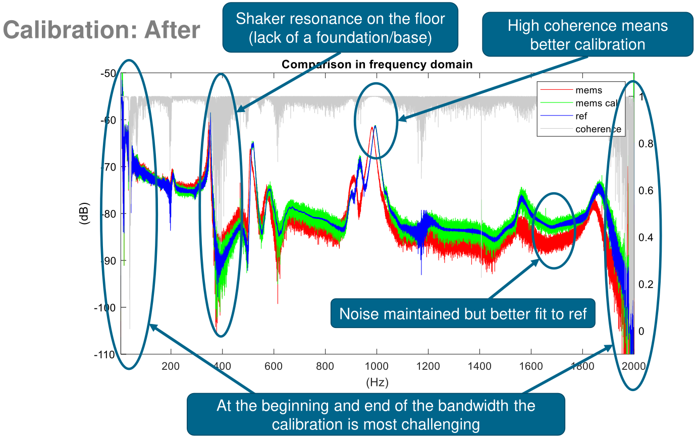
PowerPoint slide serving as a summary, taken from my PowerPoint presentation.
Quantifying calibration improvements
There are various methods for quantifying the similarity between curves like those shown in the figures. The most intuitive and direct way is to look at the correlation coefficient of uncalibrated MEMS data and calibrated MEMS data both compared to the reference data.
Due to the problematics explained in the prior paragraphs, the 0-16 Hz and 1980-2000 Hz frequency intervals are excluded from this assessment.
The following results were obtained:
- For the uncalibrated MEMS signal (red curve), the correlation coefficient of 0.832 is achieved with respect to the reference data (blue curve). This results in a deviation from the reference data of approximately 17%.
- For the calibrated MEMS signal (green curve), the correlation coefficient of 0.985 is achieved with respect to the reference data (blue curve). This results in a deviation from the reference data of approximately 1%.
While 17% is a good enough deviation to begin with, reducing it to 1% is an great result. This result is a testament to the effective test setup that could be used despite the challenges of the shaker platform’s resonance and the different accelerometer data acquisition methods that were necessary.
These results could be improved by repeating the experiments presented in this work with an improved test setup that bolts the shaker platform down. This would result in higher MEMS-reference signal coherence and possibly reduce the frequency interval that was not considered at the beginning or end, which, in this case, accounts for just 1.8% of the total frequency bandwidth.
This might not be necessary when considering the marginal improvements that would be obtained in exchange for the effort, in terms of time and licensing (namely, the VibrationView software suite), required to obtain those results.
In short, this work improved the deviation from the reference data by reducing it from 17% (uncalibrated sensor) to 1% (calibrated sensor) across 98% of the considered frequency bandwidth.
This work will hopefully help contribute to the study of microvibrations in optical laser communication terminals once the DLR CubeSat begins its in-orbit operations after launching aboard a Falcon 9 rocket in 2026.
Summary & outlook
In order to obtain accurate data on the behavior of the optical system in the vibration and micro-vibration environment generated by the in-orbit operation of the terminal itself, a calibration of the accelerometer sensor is carried out for the first time for this type of mission at DLR’s Optical Satellite Link research group.
The hardware setup used to generate and process the vibration data consists of a Vibration Research Controller connected to power amplifiers that drive the shaker platform. The Master Attitude Controller (MAC) containing the MEMS accelerometer and the reference accelerometer are excited back-to-back through a dedicated custom built interface.
For the MEMS data generation, a new state has been programmed in C++ and integrated into the MAC software codebase, allowing the direct control of the MEMS accelerometer through the terminal of a laptop running the flashing of the software and the data acquisition via a generated log file. For reference data generation, the VibrationVIEW software was used to record and export data from the reference accelerometer.
Due to the nature of the experiment and the different modes of data recording, a manual approach to data pre-processing such as time alignment of both signals has been used. The raw data were imported into Microsoft Excel, which was used to prepare CSV files for import into Matlab. In Matlab, the characterization and calibration of the MEMS sensor is performed and the Characteristic Function (CF) used to calibrate the signal is exported.
The MEMS accelerometer, which is integrated into the Master Attitude Controller (MAC) of the optical system assembly, is characterized and its behavior is compared to a reference calibrated and accurate accelerometer. The characterization includes the typical excitation approaches found in the literature, including the stepped sinusoidal approach, the chirped sinusoidal approach, and the random approach.
New Space principles of fast, cheap and modular design are being used ever more often. One example is the use of commercially off-the-shelf components (COTS) such as MEMS sensors. To ensure that the MEMS sensor is suitable for the space environment, the effect of the vibrational launch loads of the SpaceX Falcon 9 launcher, on which the satellite will be launched in 2026, and the effect of the radiation environment in LEO are investigated. It is shown that the MEMS sensor will most likely survive these conditions and remain accurate in generating the data.
After characterization, the chirped sinusoidal data is used to derive a Characteristic Function (CF) by comparison to reference data, which can be stored and used to calibrate any raw signal generated by the MEMS accelerometer. This ensures that the data generated in orbit is accurate. The successful calibration performed in this work shows an improvement in the correlation coefficient in terms of deviation from the reference data from 17% (uncalibrated) to 1% (calibrated) over 98% of the frequency bandwidth considered.
The ability to generate accurate vibration data of the in-orbit operation of the optical communications system is essential for understanding and further developing the booming sector of optical communications, with applications in satellite constellations for earth observation, connectivity or other purposes. It is hoped that this work will facilitate further development within the DLR Optical Satellite Link group, which has been at the forefront of research in this area for years, and wherever this promising technology can be exploited.
Replicate my results using my code!
An additional post is coming soon that will display all my files and provide a guide to replicate my results!
Beware: It’s Matlab heavy! :)
Bibliography
The sources I used:
Some final remarks
This post provides a brief overview of the original document, which offer a more in-depth analysis and additional topics, including investigations of Falcon 9 launch loads and the effects of end-of-life radiation on the calibration and the hardware.
Feel free to contact me if you want to take a look at the full thesis.
Ciao!